Clique Cover Problem

Here we show how to solve the clique cover problem using OpenJij, JijModeling, and ommx-openjij-adapter. This problem is also mentioned in 6.2. Clique Cover in Lucas, 2014, “Ising formulations of many NP problems”.

Overview of the Clique Cover Problem

The clique covering problem is to determine whether, given a graph and an integer \(n\), the graph can be partitioned into \(n\) cliques (complete graphs).

Complete Graph

A complete graph is a graph whose two vertices are all adjacent to each other (not including loops or multiple edges). We show two examples below.

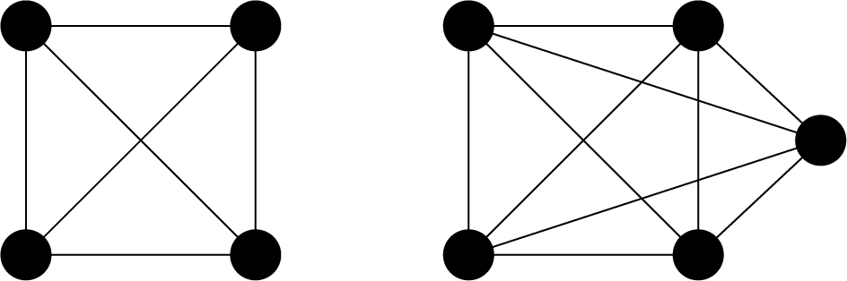
As mentioned, a vertex in a complete graph is adjacent to all other vertices. A complete undirected graph \(G = (V, E)\) has \({}_V C_2 = \frac{1}{2} V(V-1)\) edges, which shows that the number of edges is equal to the number of combinations choosing two vertices from \(V\). Based on minimizing the difference in the number of edges from a complete graph, we describe a mathematical model for the clique cover problem.

Binary Variable

We introduce a binary variable \(x_{v, n}\) such that \(x_{v, n}\) is 1 if the vertex \(v\) belongs to the \(n\)th clique and 0 otherwise.

Constraint: Each vertex can belong to only one clique

The graph is divided into \(N\) cliques:

\[ \sum_{n=0}^{N-1} x_{v, n} = 1 \quad (\forall v \in V) \tag{1} \]

Objective Function: Minimize the difference from a complete graph

Let us consider the \(n\)th subgraph. The number of vertices is \(V_n (=\sum_v x_{v, n})\). If this subgraph is complete, the number of edges is \(\frac{1}{2} V_n (V_n -1)\). The number of edges that the vertices actually form can be written as \(\sum_{(uv) \in E} x_{u, n} x_{v, n}\) using the edge set \(E\). The closer the difference between these two is to zero, the more neatly the graph is divided into cliques. Therefore, the objective function is:

\[ \mathrm{obj} = \sum_{n=0}^{N-1} \left\{ \frac{1}{2} \left( \sum_{v=0}^{V-1} x_{v, n}\right) \left( \sum_{v=0}^{V-1} x_{v, n}-1\right) - \sum_{(uv) \in E}x_{u, n} x_{v, n}\right\} \tag{2} \]

Formulation with JijModeling

Next, we show how to formulate the above mathematical model using JijModeling. We first define the variables and parameters used in the model.

import jijmodeling as jm

problem = jm.Problem('Clique Cover')

V = problem.Natural('V')
E = problem.Graph('E')
N = problem.Natural('N')
x = problem.BinaryVar('x', shape=(V, N))

Here, V is defined as the number of vertices, E as the edge set of graph \(G\), N as the number of cliques, and x is defined as a two-dimensional binary variable corresponding to \(x_{v, n}\).

Constraint

Let us formulate the constraint in equation (1).

problem += problem.Constraint('color', lambda v: jm.sum(N, lambda n: x[v, n]) == 1, domain=V)

Objective Function

Let us formulate the objective function in equation (2).

problem += jm.sum(
    N, 
    lambda n: 0.5 * jm.sum(V, lambda v: x[v, n]) * (jm.sum(V, lambda v: x[v, n])-1) - jm.sum(E, lambda e: x[e[0], n]*x[e[1], n]),
)

Let us display the formulated mathematical model in the Jupyter Notebook.

problem

\[\begin{split}\begin{array}{rl} \text{Problem}\colon &\text{Clique Cover}\\\displaystyle \min &\displaystyle \sum _{n=0}^{N-1}{\left(0.5\cdot \left(\sum _{v=0}^{V-1}{{x}_{v,n}}\right)\cdot \left(\sum _{v=0}^{V-1}{{x}_{v,n}}-1\right)-\left(\sum _{e\in E}{{x}_{{e}_{0},n}\cdot {x}_{{e}_{1},n}}\right)\right)}\\&\\\text{s.t.}&\\&\begin{aligned} \text{color}&\quad \displaystyle \sum _{n=0}^{N-1}{{x}_{v,n}}=1\quad \forall v\;\text{s.t.}\;v\in \left\{0,\ldots ,V-1\right\}\end{aligned} \\&\\\text{where}&\\&\text{Decision Variables:}\\&\qquad \begin{alignedat}{2}x&\in \mathop{\mathrm{Array}}\left[V\times N;\left\{0, 1\right\}\right]&\quad &2\text{-dim binary variable}\\\end{alignedat}\\&\\&\text{Placeholders:}\\&\qquad \begin{alignedat}{2}E&\in \mathop{\mathrm{Array}}\left[(-);\mathbb{N}\times \mathbb{N}\right]&\quad &1\text{-dimensional array of placeholders with elements in }\mathbb{N}\times \mathbb{N}\\N&\in \mathbb{N}&\quad &\text{A scalar placeholder in }\mathbb{N}\\V&\in \mathbb{N}&\quad &\text{A scalar placeholder in }\mathbb{N}\\\end{alignedat}\end{array} \end{split}\]

Creating an Instance

Let us set up the graph for clique cover.

import networkx as nx

# set the number of cliques
inst_N = 3
# set empty graph
inst_G = nx.Graph()
# add edges
inst_E = [[0, 1], [1, 2], [0, 2], 
            [3, 4], [4, 5], [5, 6], [3, 6], [3, 5], [4, 6], 
            [7, 8], [8, 9], [7, 9], 
            [1, 3], [2, 6], [5, 7], [5, 9]]
inst_G.add_edges_from(inst_E)
# get the number of nodes
inst_V = list(inst_G.nodes)
num_V = len(inst_V)
instance_data = {'N': inst_N, 'V': num_V, 'E': inst_E}

The graph set up by this instance is as follows.

import matplotlib.pyplot as plt

pos = nx.spring_layout(inst_G)
nx.draw_networkx(inst_G, pos=pos, with_labels=True)
plt.show()

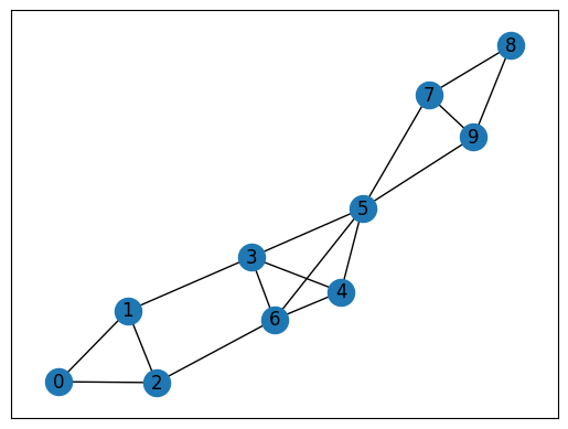
This graph consists of three cliques {0, 1, 2}, {3, 4, 5, 6}, and {7, 8, 9}. Let us verify that it can actually be divided into cliques.

Running Optimization with OpenJij

Let us solve the optimization problem using OpenJij’s simulated annealing.

from ommx_openjij_adapter import OMMXOpenJijSAAdapter

instance = problem.eval(instance_data)

adapter = OMMXOpenJijSAAdapter(instance)
best_sample = adapter.sample(
    instance, num_reads=100, uniform_penalty_weight=1.1
).best_feasible_unrelaxed

Visualizing the Solution

Let us visualize the obtained solution.

df = best_sample.decision_variables_df
x_indices = df[(df["name"] == "x") & (df["value"] > 0.5)]["subscripts"]
# initialize vertex color list
node_colors = [-1] * len(x_indices)
# set color list for visualization
cmap = plt.get_cmap("tab10")
colorlist = [cmap(i) for i in range(inst_N)]
# set vertex color list
for i, j in x_indices:
    node_colors[i] = colorlist[j]
# make figure
nx.draw_networkx(inst_G, pos=pos, node_color=node_colors, with_labels=True)
plt.show()

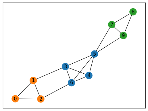
As expected, we can see that the graph is divided into three cliques.