6-量子アニーリングによる機械学習 (QBoost)
![]()
クラスタリング
クラスタリングとは与えられたデータを\(n\)個のクラスターに分けるというタスクです(\(n\)は外部から与えられているとします)。簡単のため、今回はクラスター数が2を考えましょう。
必要なライブラリのインポート
機械学習のライブラリであるscikit-learnなどをインポートします。
[1]:
# ライブラリのインポート
import numpy as np
from matplotlib import pyplot as plt
from sklearn import cluster
import pandas as pd
from scipy.spatial import distance_matrix
from pyqubo import Array, Constraint, Placeholder, solve_qubo
import openjij as oj
from sklearn.model_selection import train_test_split
人工データの生成
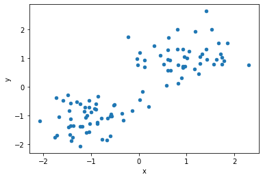
今回は人工的に二次元平面上の明らかに線形分離可能なデータを生成しましょう。
[2]:
data = []
label = []
for i in range(100):
    # [0, 1]の乱数を生成
    p = np.random.uniform(0, 1)
    # ある条件を満たすときをクラス1、満たさないときを-1
    cls =1 if p>0.5 else -1
    # ある座標を中心とする正規分布に従う乱数を作成
    data.append(np.random.normal(0, 0.5, 2) + np.array([cls, cls]))
    label.append(cls)
# DataFrameとして整形
df1 = pd.DataFrame(data, columns=["x", "y"], index=range(len(data)))
df1["label"] = label
[3]:
# データセットの可視化
df1.plot(kind='scatter', x="x", y="y")
plt.show()
今回は、以下のハミルトニアンを最小化することでクラスタリングを行います。
$:nbsphinx-math:sigma_i = \sigma_j $のとき、0
$:nbsphinx-math:sigma_i \neq `:nbsphinx-math:sigma`j :math:`のとき、`d{i,j}$
となります。右辺のマイナスに注意すると、ハミルトニアン全体では「異なるクラスに属しているサンプル同士の距離を最大にする\(\{\sigma _1, \sigma _2 \ldots \}\)の組を選びなさい」という問題に帰着することがわかります。
PyQUBOによるクラスタリング
まずは、PyQUBOで上のハミルトニアンを定式化します。そしてsolve_quboを用いてシミュレーテッドアニーリング(SA)を行います。
[19]:
def clustering_pyqubo(df):
    # 距離行列の作成
    d_ij = distance_matrix(df, df)
    # スピン変数の設定
    spin = Array.create("spin", shape= len(df), vartype="SPIN")
    # 全ハミルトニアンの設定
    H = - 0.5* sum(
        [d_ij[i,j]* (1 - spin[i]* spin[j]) for i in range(len(df)) for j in range(len(df))]
    )
    # コンパイル
    model = H.compile()
    # QUBOに変換
    qubo, offset = model.to_qubo()
    # SAで解を求める
    raw_solution = solve_qubo(qubo, num_reads=10)
    # 解を見やすい形にデコード
    decoded_sample = model.decode_sample(raw_solution, vartype="SPIN")
    # ラベルを抽出
    labels = [decoded_sample.array("spin", idx) for idx in range(len(df))]
    return labels
実行および解の確認を行います。
[20]:
labels =clustering_pyqubo(df1[["x", "y"]])
print("label", labels)
label [0, 0, 1, 0, 0, 0, 1, 0, 0, 0, 1, 0, 1, 1, 1, 0, 1, 1, 0, 1, 1, 0, 1, 1, 1, 1, 0, 1, 0, 1, 0, 0, 0, 0, 1, 1, 1, 1, 0, 1, 1, 1, 0, 0, 1, 0, 1, 1, 1, 0, 0, 1, 1, 1, 0, 0, 1, 1, 0, 0, 1, 1, 0, 1, 0, 1, 0, 0, 0, 0, 1, 0, 0, 1, 0, 0, 0, 0, 0, 1, 1, 0, 1, 0, 1, 0, 1, 0, 1, 1, 0, 1, 1, 1, 1, 1, 1, 0, 1, 0]
<ipython-input-19-42c386ac077c>:15: DeprecationWarning: Call to deprecated function (or staticmethod) solve_qubo. (You should use simulated annealing sampler of dwave-neal directly.) -- Deprecated since version 0.4.0.
  raw_solution = solve_qubo(qubo, num_reads=10)
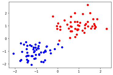
可視化をしてみましょう。
[21]:
for idx, label in enumerate(labels):
    if label:
        plt.scatter(df1.loc[idx]["x"], df1.loc[idx]["y"], color="b")
    else:
        plt.scatter(df1.loc[idx]["x"], df1.loc[idx]["y"], color="r")
Openjijのソルバーを用いたクラスタリング
次はQUBOの定式化にPyQUBOを用いて、ソルバー部分をOpenJijにしてクラスタリングを行います。
[26]:
def clustering_openjij(df):
    # 距離行列の作成
    d_ij = distance_matrix(df, df)
    # スピン変数の設定
    spin = Array.create("spin", shape= len(df), vartype="SPIN")
    # 全ハミルトニアンの設定
    H = - 0.5* sum(
        [d_ij[i,j]* (1 - spin[i]* spin[j]) for i in range(len(df)) for j in range(len(df))]
    )
    # コンパイル
    model = H.compile()
    # QUBOに変換
    qubo, offset = model.to_qubo()
    # OpenJijのSAをサンプラーに設定
    sampler = oj.SASampler(num_reads=10, num_sweeps=100)
    # サンプラーで解を求める
    response = sampler.sample_qubo(qubo)
    # 生データの抽出
    raw_solution = dict(zip(response.indices, response.states[np.argmin(response.energies)]))
    # 解を見やすい形にデコード
    decoded_sample = model.decode_sample(raw_solution, vartype="SPIN")
    # ラベルを抽出
    labels = [int(decoded_sample.array("spin", idx) ) for idx  in range(len(df))]
    return labels,  sum(response.energies)
実行および解の確認を行います。
[27]:
labels, energy =clustering_openjij(df1[["x", "y"]])
print("label", labels)
print("energy", energy)
label [1, 1, 0, 1, 1, 1, 0, 1, 1, 1, 0, 1, 0, 0, 0, 1, 0, 0, 1, 0, 0, 1, 0, 0, 0, 0, 1, 0, 1, 0, 1, 1, 1, 1, 0, 0, 0, 0, 1, 0, 0, 0, 1, 1, 0, 1, 0, 0, 0, 1, 1, 0, 0, 0, 1, 1, 0, 0, 1, 1, 0, 0, 1, 0, 1, 0, 1, 1, 1, 1, 0, 1, 1, 0, 1, 1, 1, 1, 1, 0, 0, 1, 0, 1, 0, 1, 0, 1, 0, 0, 1, 0, 0, 0, 0, 0, 0, 1, 0, 1]
energy -147945.96434710253
こちらも、可視化をしてみましょう。
[28]:
for idx, label in  enumerate(labels):
    if label:
        plt.scatter(df1.loc[idx]["x"], df1.loc[idx]["y"], color="b")
    else:
        plt.scatter(df1.loc[idx]["x"], df1.loc[idx]["y"], color="r")
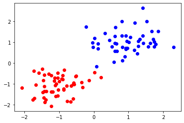
PyQUBOのSAのときと同様の結果を得ることができました。
QBoost
\(D\)個の学習データの集合を\(\{\vec x^{(d)}\}(d=1, ..., D)\)、対応するラベルを\(\{y^{(d)}\}(d=1, ..., D), y^{(d)}\in \{-1, 1\}\)とします。また、\(N\)個の弱学習器の(関数の)集合を\(\{C_i\}(i=1, ..., N)\)とします。あるデータ\(\vec x^{(d)}\) に対して、\(C_i(\vec x^{(d)})\in \{-1, 1\}\)です。このとき、最終的な分類のラベルは以下のようになります。
スクリプト
それでは実際にQBoostを試してみましょう。学習データにはscikit-learnの癌識別のデータセットを使用します。簡単のために、学習に用いるのは”0”と”1”の2つの文字種のみとします。
[30]:
# ライブラリをインポート
import pandas as pd
from scipy import stats
from sklearn import datasets
from sklearn import metrics
[31]:
# データのロード
cancerdata = datasets.load_breast_cancer()
# 学習用データと検証用データの個数の設定
num_train = 450
今回はデモンストレーションのために、ノイズとなる特徴量がある場合を考えます。
[32]:
data_noisy = np.concatenate((cancerdata.data, np.random.rand(cancerdata.data.shape[0], 30)), axis=1)
print(data_noisy.shape)
(569, 60)
[33]:
# labelを{0, 1}から{-1, 1}に変換
labels = (cancerdata.target-0.5) * 2
[34]:
# データセットを学習用と検証用に分割
X_train = data_noisy[:num_train, :]
X_test = data_noisy[num_train:, :]
y_train = labels[:num_train]
y_test = labels[num_train:]
[35]:
# 弱学習器の結果から
def aggre_mean(Y_list):
    return ((np.mean(Y_list, axis=0)>0)-0.5) * 2
弱学習器の作成
scikit-learnで弱分類器を作成します。今回は弱分類器としてdecision stumpを用いましょう。decision stumpとは、一層の決定木のことです。今回は弱分類器として用いるので、分割に用いる特徴量はランダムに選ぶこととします(一層のランダムフォレストを行うという理解で良いでしょう)。
[36]:
# 必要なライブラリのインポート
from sklearn.tree import DecisionTreeClassifier as DTC

# 弱分類機の個数の設定
num_clf = 32
# bootstrap samplingで、一つのサンプルに対して取り出すサンブル個数
sample_train = 40
# モデルの設定
models = [DTC(splitter="random",max_depth=1) for i in range(num_clf)]
for model in models:
    # ランダムに抽出
    train_idx = np.random.choice(np.arange(X_train.shape[0]), sample_train)
    # 説明変数と目的変数から決定木を作成
    model.fit(X=X_train[train_idx], y=y_train[train_idx])
y_pred_list_train = []
for model in models:
    # 作成したモデルを用いて予測を実行
    y_pred_list_train.append(model.predict(X_train))
y_pred_list_train = np.asanyarray(y_pred_list_train)
y_pred_train =np.sign(y_pred_list_train)
すべての弱学習器を最終的な分類器としたときの精度を見てみましょう。以後、この組み合わせをbaselineとします。
[37]:
y_pred_list_test = []
for model in models:
    # 検証データで実行
    y_pred_list_test.append(model.predict(X_test))

y_pred_list_test = np.array(y_pred_list_test)
y_pred_test = np.sign(np.sum(y_pred_list_test,axis=0))
# 予測結果の精度のスコア計算
acc_test_base = metrics.accuracy_score(y_true=y_test, y_pred=y_pred_test)
print(acc_test_base)
0.9327731092436975
[38]:
# QBoostを行うクラスを定義
class QBoost():
    def __init__(self, y_train, ys_pred):
        self.num_clf = ys_pred.shape[0]
        # バイナリ変数を定義
        self.Ws = Array.create("weight", shape = self.num_clf, vartype="BINARY")
        # 正規化項の大きさ(ハイパーパラメータ)をPyQUBOのPlaceholderで定義
        self.param_lamda = Placeholder("norm")
        # 弱分類器の組み合わせのハミルトニアンをセット
        self.H_clf = sum( [ (1/self.num_clf * sum([W*C for W, C in zip(self.Ws, y_clf)])- y_true)**2 for y_true, y_clf in zip(y_train, ys_pred.T)
        ])
        # 正規化項のハミルトニアンを制約としてセット
        self.H_norm = Constraint(sum([W for W in self.Ws]), "norm")
        # 全ハミルトニアンをセット
        self.H = self.H_clf + self.H_norm * self.param_lamda
        # モデルをコンパイル
        self.model = self.H.compile()
    # QUBOに変換する関数を定義
    def to_qubo(self, norm_param=1):
        # ハイパーパラメータの大きさを設定
        self.feed_dict = {'norm': norm_param}
        return self.model.to_qubo(feed_dict=self.feed_dict)
[39]:
qboost = QBoost(y_train=y_train, ys_pred=y_pred_list_train)
# lambda=3としてQUBO作成
qubo = qboost.to_qubo(3)[0]
D-Waveサンプラーを用いてQBoostを実行
[ ]:
# 必要なライブラリをインポート
from dwave.system.samplers import DWaveSampler
from dwave.system.composites import EmbeddingComposite
[ ]:
dw = DWaveSampler(endpoint='https://cloud.dwavesys.com/sapi/',
                  token='xxxx',
                  solver='DW_2000Q_VFYC_6')
sampler = EmbeddingComposite(dw)
[ ]:
# D-Waveサンプラーで計算
sampleset = sampler.sample_qubo(qubo, num_reads=100)
[ ]:
# 結果の確認
print(sampleset)
[ ]:
# 各計算結果をPyQUBOでdecode
decoded_solutions = []
brokens = []
energies =[]

decoded_sol = qboost.model.decode_dimod_response(sampleset, feed_dict=qboost.feed_dict)
for d_sol, broken, energy in decoded_sol:
    decoded_solutions.append(d_sol)
    brokens.append(broken)
    energies.append(energy)
D-Waveで得られた弱分類器の組み合わせを使った場合の、学習データ/検証データでの精度を確認しましょう。
[ ]:
accs_train_Dwaves = []
accs_test_Dwaves = []
for decoded_solution in decoded_solutions:
    idx_clf_DWave=[]
    for key, val in decoded_solution["weight"].items():
        if val == 1:
            idx_clf_DWave.append(int(key))
    y_pred_train_DWave = np.sign(np.sum(y_pred_list_train[idx_clf_DWave, :], axis=0))
    y_pred_test_DWave = np.sign(np.sum(y_pred_list_test[idx_clf_DWave, :], axis=0))
    acc_train_DWave = metrics.accuracy_score(y_true=y_train, y_pred=y_pred_train_DWave)
    acc_test_DWave= metrics.accuracy_score(y_true=y_test, y_pred=y_pred_test_DWave)
    accs_train_Dwaves.append(acc_train_DWave)
    accs_test_Dwaves.append(acc_test_DWave)
横軸をエネルギー、縦軸を精度のグラフを作成しましょう。
[ ]:
plt.figure(figsize=(12, 8))
plt.scatter(energies, accs_train_Dwaves, label="train" )
plt.scatter(energies, accs_test_Dwaves, label="test")
plt.xlabel("energy: D-wave")
plt.ylabel("accuracy")
plt.title("relationship between energy and accuracy")
plt.grid()
plt.legend()
plt.show()
[ ]:
print("base accuracy is {}".format(acc_test_base))
print("max accuracy of QBoost is {}".format(max(accs_test_Dwaves)))
print("average accuracy of QBoost is {}".format(np.mean(np.asarray(accs_test_Dwaves))))
D-Waveによるサンプリングは短時間で数百サンプリング以上が実行できます。精度が最大になる結果を使えば、baselineよりも高精度の分類器を作成することが可能です。