A1 - Introduction to OpenJij core interface (core Python interface)¶

In this chapeter, let us show you how to use OpenJij core interface (core Python insterface) and demonstrate easy case of calculation.

Core insterface is lower-layer APIs than in the previous tutorials. The target readers are expected to have completed the previous OpenJij tutorials and be familiar with terms such as ising models and MonteCarlo methods.

Specifically, we use OpenJij for the following purpose.

We would like to use OpenJij not only for optimization problems, but also for more specialized applications such as sampling and research purpose.
We would like to set annealing schedules and directly develop algorithms we use.

About OpenJij core interface¶

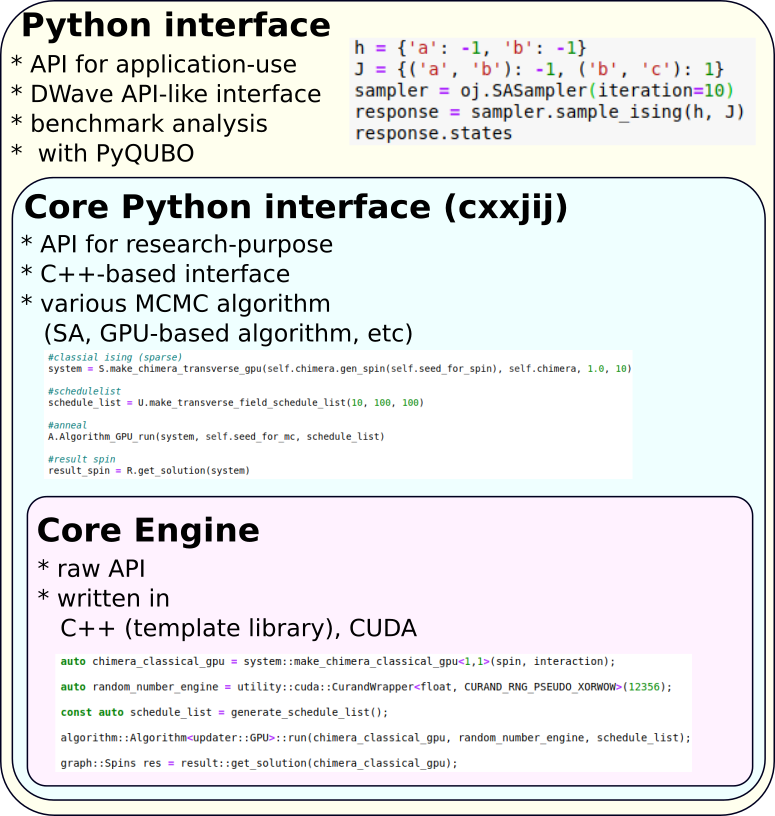
In previous tutorial, we introduced how to solve various problems and how to benchmark with OpenJij. The lowest level of OpenJij is implemented in C++ based on the Markov Chain MonteCarlo (MCMC) method for statistical physics numerical scheme. The Python modules of OpenJij call cxxjij, a Python library that wraps this C++ interface directly. The figure show the following inclusion relaationship.

Using core interface, we can use all funtinon of OpenJij. Therefore, We can choose OpenJij not only for optimization problem but also for reserch purpose as numerical tools of statistical physics. Also, we can compute faster computation because of using C++ interface.

In this tutorial, let us introduce you Python interface cxxjij and C++ interface. We use pip for installation.

[ ]:

!pip install openjij
!pip show openjij

Run problem¶

As a tutorial, we solve classical spin-ising problem (\(\sigma = \pm 1\)) with \(N=5\) variable size with annealing. The Hamiltonian of this problem is as follows.

\begin{align} H &= \sum_{i

When the longitudinal magnetic fields and interaction coefficient are as follows

\begin{align} h_i = -1 \ \mathrm{for\ } \forall i,\ J_{ij} = -1　\ \mathrm{for\ } \forall i,\ j \end{align}

all spin is lower in energy if it takes a value of 1. Therefore, the optimal solution is \(\{\sigma_i\} = \{1,1,1,1,1\}\). Let’s solve this problem.

The whole process with the Python script is as follows.

core interface is a solver that specializes in ising problem. For this reason, conversion with QUBO is not implemented. To convert to QUBO, please refer to the previous tutorials and convert from QUBO to Ising problem before calling the core interface.

[2]:

# core interface imports cssjij instead of OpenJij
import cxxjij as cj
# import Graph module for interaction matrix
import cxxjij.graph as G

# set Dense Graph of problem size N=5
N = 5
J = G.Dense(N)
# set interaction matrix
for i in range(N):
    for j in range(N):
        J[i,j] = 0 if i == j else -1.0
# set longitudinal matnetic fields
for i in range(N):
    # we can get same result J[i,i] = -1
    J[i] = -1

# import system to perform the computation from Graph
import cxxjij.system as S

# In this time, we use normal classical MonteCarlo calculation system
system = S.make_classical_ising(J.gen_spin(), J)
# use Utility to set annealing schedule
import cxxjij.utility as U
schedule = U.make_classical_schedule_list(0.1, 100, 10, 10)

# use Altorigthm to run annealing
# use simple SingleSpinFlip for updating the MonteCarlo step
import cxxjij.algorithm as A
A.Algorithm_SingleSpinFlip_run(system, schedule)

# use get_soultion in Result module to get result
import cxxjij.result as R
print("The solution is {}.".format(R.get_solution(system)))

The solution is [1, 1, 1, 1, 1].

We can see this solution is \([1,1,1,1,1]\). Because it is a low layer API, there are many settings to be made, but the more detailed settings are possible.

List of Modules¶

As a script example, OpenJij core interface consists of graph, system, algorigthm and other modules. Each module can be combined to compute ising models of various types and algorithms. It is also easy to extend when implementing new algorithms. The following chapters will explain details.

Graph¶

A module for holding the ising Hamiltonian’s coefficient \(J_{ij}\). There are Dense and Sparse, which deal with tight coupling (suitable for models in which all Jij have non-zero values) and others (suitable for models in whick many Jij values are zero).

System¶

system defines a data structure for keeping the current status of the system in MonteCarlo simulation and others.

Specifically, the following are defined.

Classical ising model (sequence of spins)
Ising model including transverse magnetic fields (sequence of spins including Trotter decomposition)
GPU implemented classical and quantum ising model

There are many different MonteCarlo methods and other computation schemes (or new methods will be developed in the feature). Therefore, by separating the data structures, algorithms and result fetching interfaces for each methods, OpenJij has been designed to make it easy to add different algorithms.

Updater¶

updater difines how to update the system. Specifically, the following methods are implemented.

SingleSpinFlip Update
SwendsenWang Update

system type determines which updater can be used.

In core python interface, updater is integrated into the algorithm.

Algorithm¶

Algorithm has a role of executing altorighms, including what schedule to run the annealing algorithm. Algorithm_[Updater_type]_run allows you to run the program using the corresponding Updater.

Result¶

This module is used to get information from the system such as spin assignment.

Coding Flow¶

The coding process is basically as fllows. This trend will not change as the scale of the problem is largeer.

set \(J_{ij}, h_{i}\) with graph
create system based on graph
select updater for the system and run the algorithm using Algorithm_[Updater type]_run
get system spin assignment with result.get_solution(system) or get from system directly.