How to use the standard error function of benchmark functions

This section explains how to use the standard error function added to the benchmark function.

Install Libraries and model preparation

We can branch an additional feature/error_bar repository into own repository, which we forked from OpenJij’s repository.

Antiferomagnetic one-dimensional Ising model preparation,

import random
import numpy as np
import matplotlib.pyplot as plt
import openjij as oj

# set antiferomagnetic one-dimensional Ising model
N = 30
h = {0: -10}
J = {(i, i+1): 1 for i in range(N-1)}

Benchmark function

The usage is the same as before.

Auguments are unchanged. The following calculations are now stored in a new dictionary type as the return value.

• se_success_prob: a list of standard errors for success probability

  standard deviation of the expected value of success probability when we anneal iteration times. the values are stored for each step_num
• se_residual_energy: a list of standard errors for residual energy

  standard deviation of the average value of residual energy when we anneal iteration times. the values are stored for each step_num

• se_lower_tts: a list of lower errors in TTS The lower error of TTS computed based on the upper error of success probability

• se_upper_tts: a list of upper errors in TTS The upper error of TTS computed based on the lower error of success probability

# set optimal solution
correct_state = [(-1)**i for i in range(N)]

# set step_num and iteration
step_num_list = list(range(10, 101, 10))  # [10, 20,,,, 100]
iteration = 100

# compute TTS, residual energy, success probability, specimen average & standard error
sampler = oj.SASampler(num_reads=iteration)
result = oj.solver_benchmark(
                      solver=lambda time, **args: sampler.sample_ising(h,J,num_sweeps=time),
                      time_list=step_num_list, solutions=[correct_state], p_r=0.99
            )

# option: seaborn is good at visualization
# !pip install seaborn
import seaborn as sns
sns.set()

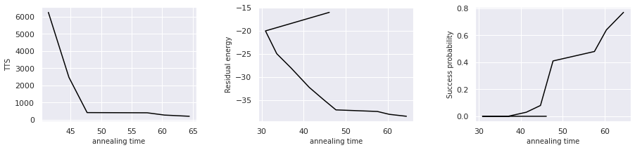
TTS, residual energy and success probability

We can visulalize TTS, residual energy, success probability as before.

fig, (axL,axC,axR) = plt.subplots(ncols=3, figsize=(15,3))
plt.subplots_adjust(wspace=0.4)

fontsize = 10
axL.plot(result['time'], result['tts'], color = 'black')
axL.set_xlabel('annealing time', fontsize=fontsize)
axL.set_ylabel('TTS', fontsize=fontsize)

axC.plot(result['time'], result['residual_energy'], color = 'black')
axC.set_xlabel('annealing time', fontsize=fontsize)
axC.set_ylabel('Residual energy', fontsize=fontsize)

axR.plot(result['time'], result['success_prob'], color = 'black')
axR.set_xlabel('annealing time', fontsize=fontsize)
axR.set_ylabel('Success probability', fontsize=fontsize)

Text(0, 0.5, 'Success probability')

Standard error

The value of standard error is stored in se_success_prob & se_residual_energy. These allow us to display standard error bars.

# check for standard errors
print(result['se_upper_tts'])
print(result['se_lower_tts'])
print(result['se_residual_energy'])
print(result['se_success_prob'])

[inf, inf, inf, inf, 7695.650221419744, 3644.8655556701647, 3208.0260160559314, 14055.445317726388, 1322.6002725331891, 489.1079299082817]
[inf, inf, inf, inf, 5398.579224570907, 1993.1589254329997, 321.5840555508159, 337.1023745696516, 272.15911680620405, 201.95995978525684]
[4.869986414433583, 4.426686746942408, 3.9944911560747753, 3.4523597551222673, 3.5046866169214455, 2.512112073675669, 2.0192007619777974, 1.906925178491185, 1.4905764595679691, 1.1399096189584241]
[0.0, 0.0, 0.0, 0.0, 0.17058722109231983, 0.2712931993250107, 0.49183330509431744, 0.4995998398718718, 0.48, 0.4208325082500163]

# visualization
fig, (axL,axC,axR) = plt.subplots(ncols=3, figsize=(15,3))
plt.subplots_adjust(wspace=0.4)

fontsize = 10
axL.plot(result['time'], result['tts'])
axL.errorbar(result['time'], result['tts'], yerr = (result['se_lower_tts'],result['se_upper_tts']), capsize=5, fmt='o', markersize=5, ecolor='black', markeredgecolor = "black", color='w')
axL.set_xlabel('annealing time', fontsize=fontsize)
axL.set_ylabel('TTS', fontsize=fontsize)

axC.plot(result['time'], result['residual_energy'])
axC.errorbar(result['time'], result['residual_energy'], yerr = result['se_residual_energy'], capsize=5, fmt='o', markersize=5, ecolor='black', markeredgecolor = "black", color='w')
axC.set_xlabel('annealing time', fontsize=fontsize)
axC.set_ylabel('Residual energy', fontsize=fontsize)

axR.plot(result['time'], result['success_prob'])
axR.errorbar(result['time'], result['success_prob'], yerr = result['se_success_prob'], capsize=5, fmt='o', markersize=5, ecolor='black', markeredgecolor = "black", color='w')
axR.set_xlabel('annealing time', fontsize=fontsize)
axR.set_ylabel('Success probability', fontsize=fontsize)

Text(0, 0.5, 'Success probability')

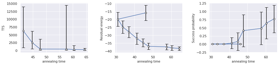
As annealing time per session increased, error bars of the standard errors for success probability and residual energy become shorter and shorter.